Functions, Formatting, Filtering

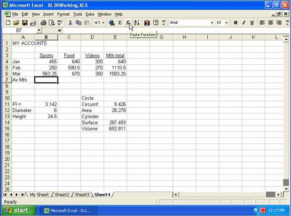
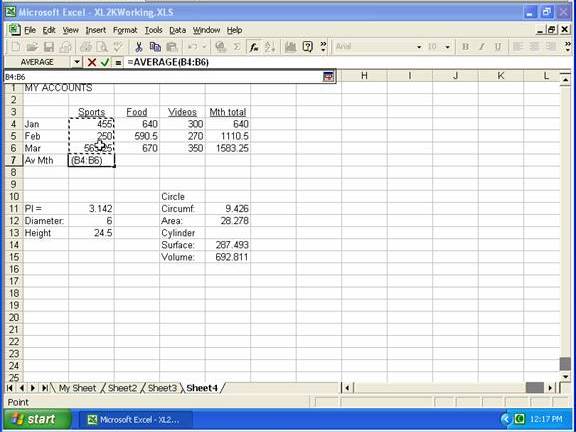
To add a function (such as AVERAGE), click Paste Function button …

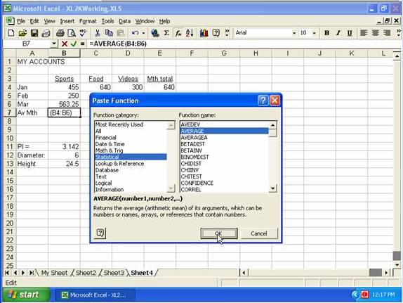
… select the required Function category …

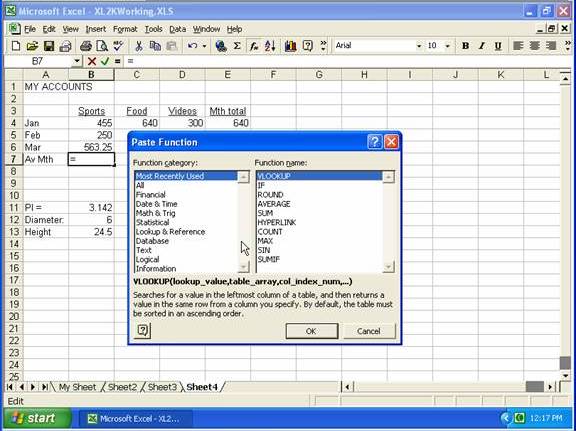
… then select the required function (in this case Average), then click OK.

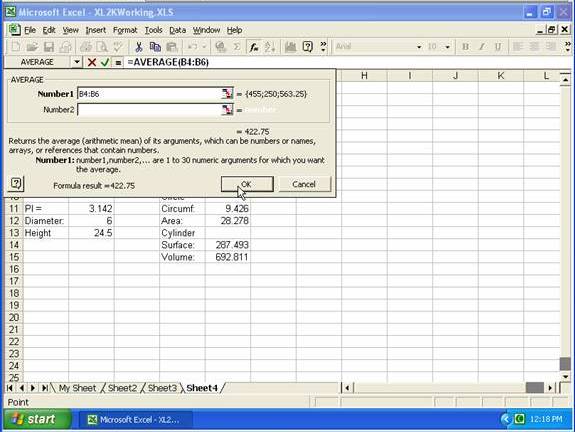
You will then get a window to construct the function, and in this example you could directly enter the range to get the average of, or you could click Collapse button …

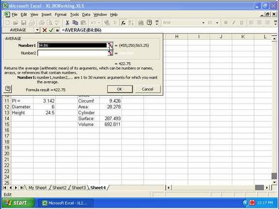
… select the cells required, then click the Expand button (or press Enter) …

… then click OK.

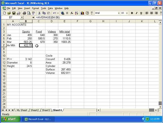
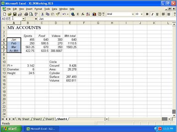
Below you can see the actual function that gets entered in the cell (you could have typed =AVERAGE(B4:B6) directly and got the same result)

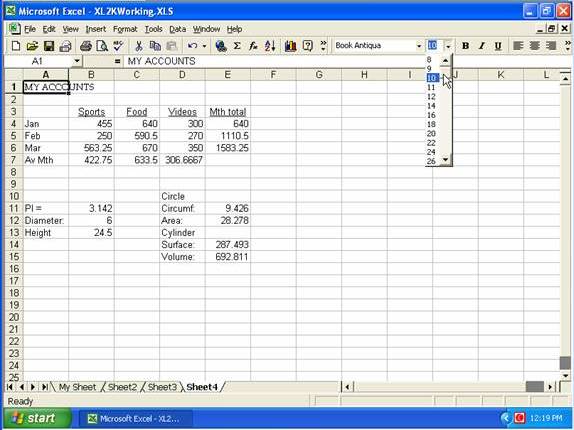
To change the font type, click Font arrow on toolbar, select the required type from the Font drop-down list.

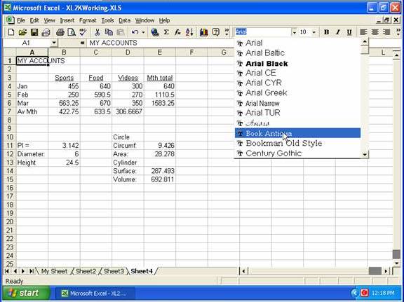
You can change the size of the font from the Font Size list.

To apply the format of one cell to another, select the cell (or cells) with the required font, click Format Painter …

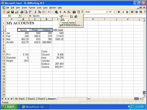
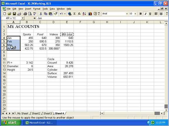
… then click on the cell to receive the formatting.

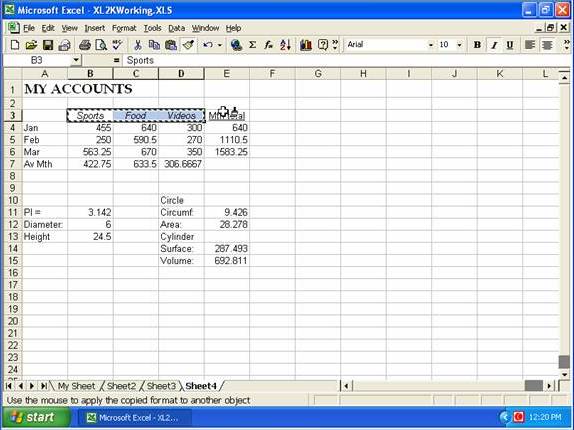
Double-clicking on Format Painter button (mouse changes to paintbrush) will allow you to apply the format of the originally selected cell to a number of cells. Press ESC to turn off format painter.

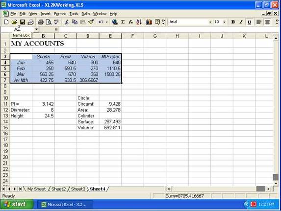
Typing a range of cells in the Name Box and pressing Enter …

… will select that range of cells.

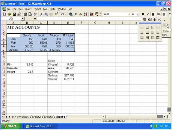
With a block of cells selected you can click the Borders drop-arrow on the Formatting toolbar …

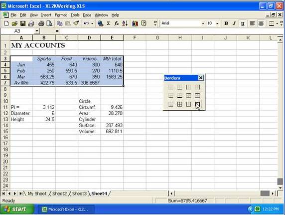
… and drag the borders palette to convenient spot (if necessary), click the required border button, then click the close button [X] on the Borders palette to close it (if you have dragged it loose of the borders button).

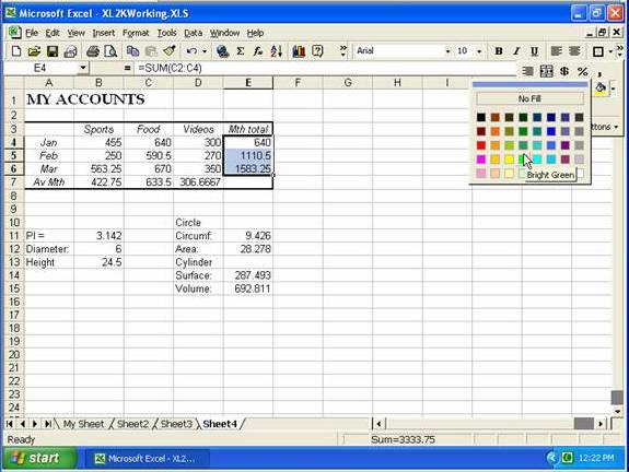
To apply a background color to one or more selected cells, click the Fill Color drop-arrow on the toolbar and select the required color

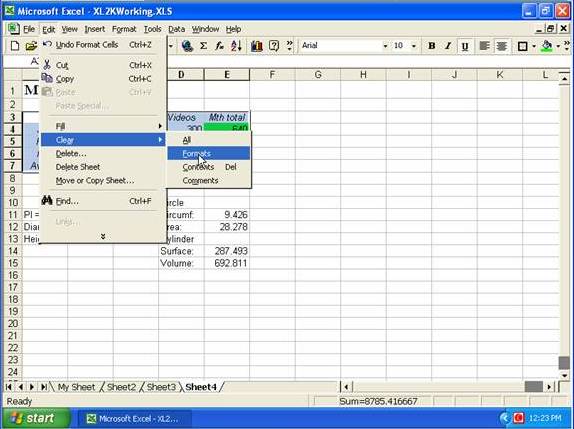
To remove the formatting from selected cells, go to the Edit menu, Clear, Formats.

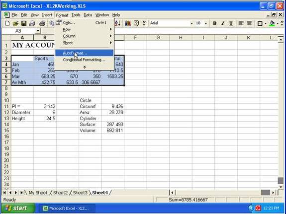
A quick way to apply formatting is to go to the Format menu and select AutoFormat …

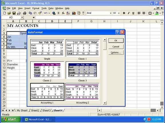
… select the option required, then click OK.

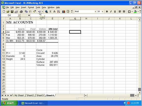
To remove the formatting just applied, click the Undo button.

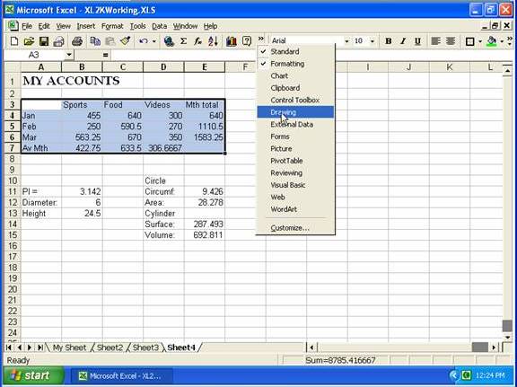
Right-clicking on a toolbar will show the list of available toolbars, and here we are selecting the Drawing toolbar.

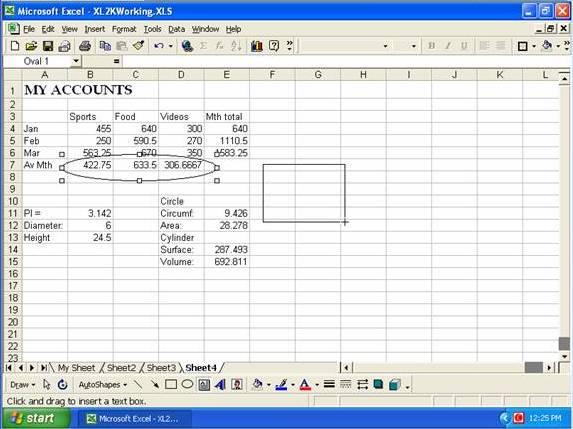
Then you could click on the Oval tool, drag out an overall over some entries you want to identify …

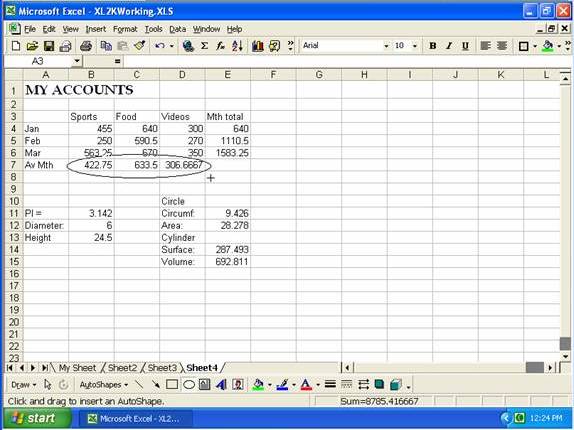
… move the oval over the required cells, if necessary, …

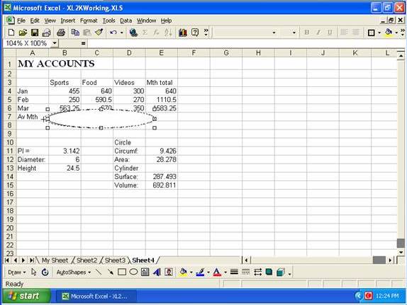
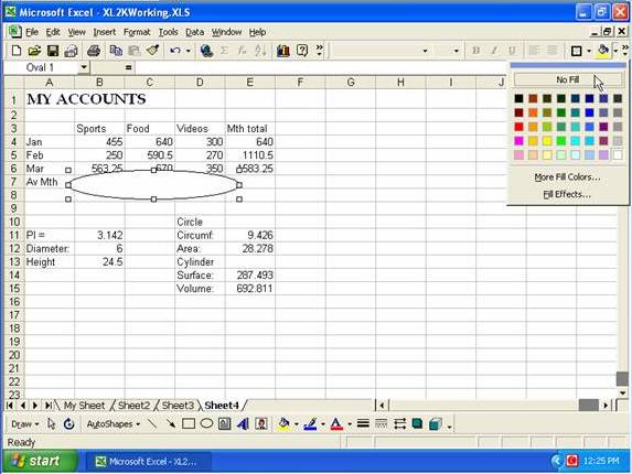
… then click on the Fill Color drop-arrow and select No Fill …

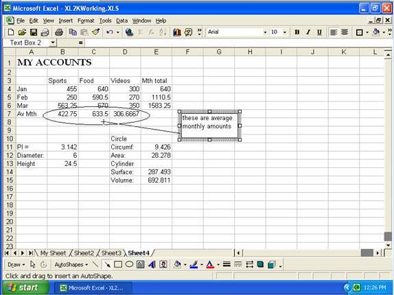
You could click on the Text Box tool (on the Drawing toolbar), drag out the text box, type the required text …

… then you could click the Arrow tool (on the Drawing toolbar), click at mid-point of left side of text box, and drag to the oval.

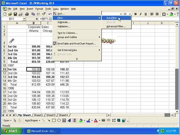
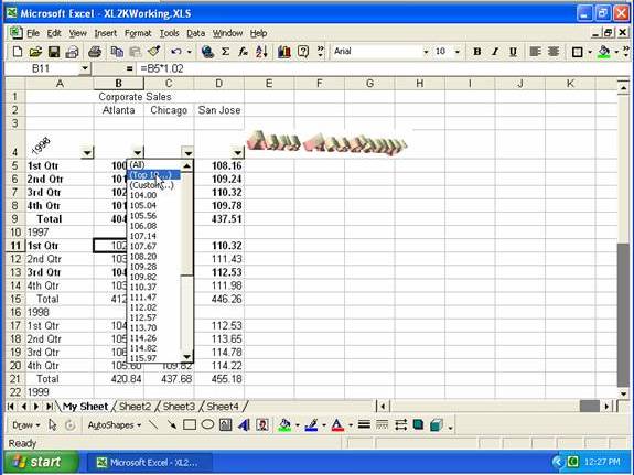
To set up a spreadsheet so you can filter the entries, go to the Data menu, select Filter, then AutoFilter (to turn it on) …

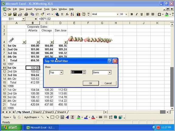
Then you can select individual values to filter on, or options such as Top 10 …

… and you could then adjust that …

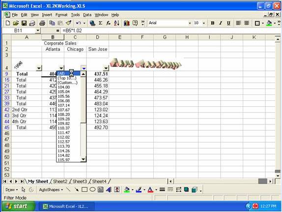
… selecting (All) will redisplay all the entries

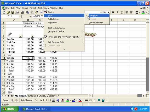
To turn off AutoFilter, go to the Data menu, select Filter, and click AutoFilter again.